Symbolic Graph Reasoning Meets Convolutions

The last author of this paper is Eric P. Xing, which is my idol. And i have hounor to see him in Sanya early in this year. This paper is the newest work advanced by him and published on Neurips 2018.

Symbolic Graph Reasoning Meets Convolutions

---

The proposed method is illustrated below:

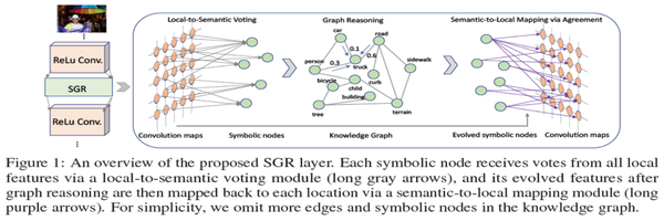
It is composed of three parts, we will dig out these components one by one.

PART I: Local-to-Semantic Voting Module

Purpose:

Given local feature tensors from convolution layers, our target is to leverage global graph Reasoning to enhance local features with external structured knowledge.

keywords: voting matrix

How to do:

First summarize the global information encoded in local features into representations of Symbolic nodes. The procedure of this part is marked by green box below:

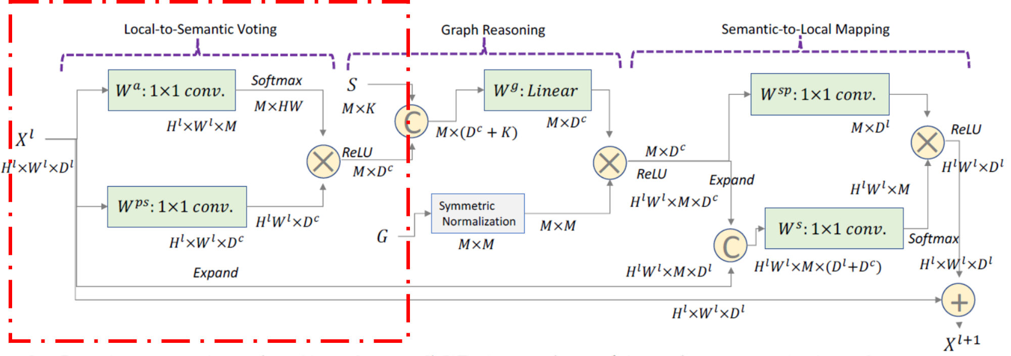
This module aims to produce visual representations $ H^{p s} \in \mathbf{R}^{M \times D^{c}} $ of all $ M =

\mathcal{N}

$ symbolic nodes using $ X^{l} $, where $ D^{c} $ is the desired feature dimension for each node $ n $, which is formulated as the function $ \phi $ below:

$$H^{p s}=\phi\left(A^{p s}, X^{l}, W^{p s}\right)$$

$ X^{l} \in \mathbf{R}^{H^{l} \times W^{l} \times D^{l}} $ represents the feature tensor after $ lth $ convolution layer as the module inputs, where $ H^{l} $ and $ W^{l} $ are height and weight of feature maps while $ D^{l} $ is the channel number.

$ W^{p s} \in \mathbf{R}^{D^{l} \times D^{c}} $ is the trainable transformation matrix for converting each local feature $ x_{i} \in X^{l} $ into the dimension $ D^{c} $.

$ A^{p s} \in \mathbf{R}^{H^{l} \times W^{l} \times M} $ denotes the voting weights of all local features to each symbolic node.

More specifically, the function $ \phi $ is computed as follows:

$$H_{n}^{p s}=\sum_{x_{i}} a_{x_{i} \rightarrow n} x_{i} W^{p s}$$ $$a_{x_{i} \rightarrow n}=\frac{\exp \left(W_{n}^{a T} x_{i}\right)}{\sum_{n \in \mathcal{N}} \exp \left(W_{n}^{a T} x_{i}\right)}$$

Here $ W_{n}^{a} \in \mathbf{R}^{D^{l}} $ is a trainable weight matrix for calculating voting weights. It’s convenient to know that $ a_{x_{i} \rightarrow n} \in \mathbf{R}^{1} $, when go through all of the local features $x_{i}$, where $ i=1,…,H \times W $, and all of the $ a_{x_{i} \rightarrow n} $ components the $ A^{p s}_{n} \in \mathbf{R}^{H \times W} $ (we omit upper label $ l $ for convenience) for the $ nth $ symbolic node.

Please note that $ W^{p s} $ is a global trainable parameter while $ W^{a} $ is a local trainable parameter which contains n components $ W^{a}_{n} $ tranversing all symbolic nodes.

That’s why in the last sentence of the section says “In this way, different local features can adaptively vote to representations of distinct symbolic nodes.”

PART II: Graph Reasoning Module

Purpose:

Based on visual evidence of symbolic nodes, the reasoning guided by structured knowledge is employed to leverage semantic constraints from human commonsense to evolve global representations of symbolic nodes.

keywords: propogation rule, adjacency matrix

How to do:

We incorporate both linguistic embedding of each symbolic node and knowledge connections for performing graph reasoning. The procedure of this part is marked by blue box below:

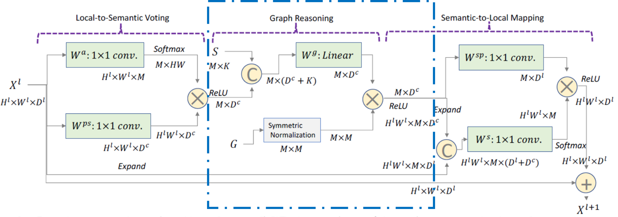
Concretely speaking, for each symbolic node $ n \in \mathcal{N} $, we use fasttext (the off-the-shelf word vectors) as its linguistic embedding, denoted as $ \mathcal{S}={s_{n}} $, where $ s_{n} \in \mathbf{R}^{K} $. As for edges, we need to look at its propogation rule. The graph reasoning module performs graph propogation over representations $ H^{p s} $ of all symbolic nodes via the matrix multipulation form, resulting in the evolved features $ H^{g} $:

$$H^{g}=\sigma\left(A^{g} B W^{g}\right)$$

Here $ B=\left[\sigma\left(H^{p s}\right), \mathcal{S}\right] \in \mathbf{R}^{M \times\left(D^{c}+K\right)} $ concat features of transformed $ H^{p s} $ via the function $ \sigma(.) $ and the linguistic embedding $ \mathcal{S} $.

$ W^{g} \in \mathbf{R}^{\left(D^{c}+K\right) \times\left(D^{c}\right)} $ is a trainable weight matrix.

The node adjacency weight $ a_{n \rightarrow n^{\prime}} \in A^{g} $ is defined according to the edge connections in $ \left(n, n^{\prime}\right) \in \mathcal{E} $ (Here adjacency matrix is predefined). The edge connections can be soft weights (e.g. 0.8) or hard weights ({0, 1}) according to different knowledge graph resources.

Further more, we add the self-loop as well as norm $ A^{g} $ inspired from GCNs. The overall formulation arrives in: